The sBitx – The SDR for the homebrewer
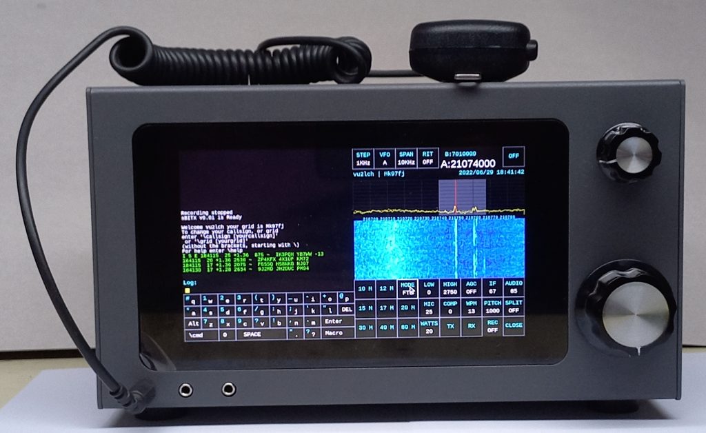 The sBitx is a homebrewer’s SDR radio with integrated digital modes.
- Maximum power output of 40 watts on 80M and 40M bands, goes down to 20 watts on 15M and 6 watts on 10M.
- Based on a Raspberry Pi, a WM8731 codec and ordinary components found in your junkbox
- Uses a hybrid superhet architecutre for high performance design
- You can build it for less than $100 in new parts in addition to the Raspberry Pi and Display.
- The circuit is simple to build without any FPGAs and expensive parts
- The software is hackable, modular.
- Download circuit diagram and software from https://github.com/afarhan/sbitx
- Here is the Raspberry Pi Image for the sBitx. Download, unzip and burn it into a 32GB SD card.
- Read the Operating Manual (it is frequencly updated, don’t download and print!)
Why should we homebrew an SDR?
It is a good question. Considering that the author devoted most of his last five years to building and writing one, there should be a legitimate answer to this.Because it is there
Was it George Mallory who, whe was asked why he wanted to summit Everest, replied “Because it is there”? I am reminded of the work that early transistor pioneers like Wes Hayward, W7ZOI and Doug Demaw, W1FB did for the transistors. At that time, the transistors were unwieldy beasts, fragile and confusing. They had no similarity with the valves that were prevalent at the time. Their series of articles in the QST culminated in the book Solid State Design for the Radio Amateur. It changed everything and made the new technology accessible and easy. Furthermore, the prices dropped, valves went out of stock and the world became transistorized very quickly. The radio amateurs were already there. Does this mean that the old analog radio is dead? Well, not at all. Analog electronics is the basis of all radio science, even the software defined radios. This project proves that our learning from the conventional superhet radio engineering can well be applied to the SDRs. Increasingly, more and more radios will be built with software defined architectures. We must bring our craft right into the cutting edge of contemporary science rather than the trailing edge; especially when it comes laden with gifts. Running CW on an SDR is perfect joy. Especially if it is a radio that you have made all by yourself. The filtering is ring-free; the sending is perfect with the macros and a computer keyboard, logging is transparent, recording your brag tapes happens with a touch, adding quirky features does not require you to drill holes in the front-panel or soldering!The Learning
A large part of our hobby is to constantly learn new stuff. Amazingly, age is on your side.. The experience with building and using our equipment makes us better with age (Guilty as charged, I am on the better side of the 50s). However, when I set out to study software defined radios, unlike staring at a circuit and ‘getting it’ within minutes, I realized that the software was thousands of lines of code, usually written to get the job done rather than to explain the job being done. It was impossible to study it, let alone modify or borrow from any of them. Hence, the need to write a new SDR that is easily understood and adapted, modified and extended to do more and more exciting things. You can think of the sBitx as a stable start of your learning of the SDR. It has certainly been for the author who started with Zilch. The main source code to receive and transmit fit into a single page (just like a QRP radio’s circuit would), the actual circuit can be put together, from your junkbox!Budget Performance
Usually, it takes a large investment and lots of time and work to build a station that matches a commercial radio. The fancy radios available for thousands of dollars has all the knobs and buttons that allow you to do smart things that make life simple. However, behind that front panel, everything is software, and the software can be free! That’s the hidden beauty of a software defined radio. Consider that you built a super simple SSB rig, like Pete Juliano, N6CQ’s PSST(https://www.n6qw.com/PSSST_20.html), It has all of seven devices. Now consider adding variable bandwidth filters, AGC, upper and lower sidebands, other voice modes, CW, RTTY, even FT8. The project will look enormous! However, it can all be added with just a Raspberry Pi and an audio chip! Instead of looking at SDR as an expensive, complex approach to building radios, think of it as an easy way to add all the features of a professionally produced radio for no extra circuitry! With the SDRs, the homebrewer can finally build radios that are as feature laden as the commercial radios, customize them to their hearts’ content and do it at a fraction of the cost of commercial radios.Works the world from anywhere
Our last argument for an integrated SDR like the sBitx is that it allows you to quickly setup a station from anywhere without the entire paraphernalia of cables, computer interfaces, etc. and work the world on less than optimal antennas like mag-loops and whips because of the amazing software that works at digging signals right out of noise! Setting up a station with loggers, data software like WSJT-X, Fldigi and homebrew radios is a mess of wires, configuration files and things going wrong. An integrated radio like the sBitx is a first. Everything comes pre configured on a single SD card. It is built to a particular digital hardware (the Raspberry Pi with a stereo 96 ksps codec). Just switch on and go!The Hybrid SDR
The central challenge to building an acceptable SDR radio is to choose an architecture and circuitry that will eliminate the image. For phasing SDR radios the image is just a few tens of KHz away, creating ghost signals. For direct conversion radios, the spurious responses are determined by the number of usable bits in the analog to digital and digital to analog conversion circuits. These can be very expensive and very hard to build in the homelab. Typically these ADC have ball grid array pads below them that can only be soldered properly by pick and place machines. Engineering is the art of compromise with science. It is where the practical considerations meet the hard truth of mathematics of physical laws. The Hybrid SDR solves the image problem using the best analog way available: Use an aggressive crystal filter in a superhet architecture.. The hybrid approach to SDRs is a huge gain in terms of ease of build, performance. This compromise is the width of the waterfall : the sBitx limits itself to a maximum of 25 KHz of spectrum scope.Is 25 KHz waterfall enough?
Those used to watching the waterfall of an entire band may think this is a limiting factor. Actually, it is not. Most of the CW operators, even in contests, operated within 10 KHz span at a time. This makes it easy to see closely spaced signals that will get clustered too closely even at 25 KHz widths. Much of DX hunting and expeditions happens in very small windows in a band. The digital modes like the FT8 or JS8Call limit themselves to within 3 KHz. So, even 10 KHz of waterfall is wasted on them. In a contest, if you are running (Calling CQ and waiting for others to return your call) you just stick to one frequency and listen a few kilohertz up and down. If you are tuning around in a contest, picking up the weak signals, it is best to have a magnified waterfall to see the faint traces of the individual signals.The Up-converting superhet
The sBitx is an up-converting superhet with the IF at 40 MHz. This eliminates the need for multiple filters, one for each band of operation. As our frequencies of interest are below 30 MHz and the local oscillator is above 40 MHz, the image frequencies are well above 80 MHz. These are easily filtered by a simple low pass filter for the entire HF band. Central to the approach of the sBitx is that we can build a 25 KHz width crystal filter that has a very sharp image rejection. This is now possible with the easily available, low cost 40 MHz fundamental mode crystals (ABM10AIG-40.000MHZ-2Z-T from Mouser.com).Homebrew-ability
With a superhet architecture, we can use our familiar techniques of building one in multiple ways. From using diode mixers and bipolar transistors to using passive FET front-ends without early amplifiers, these can be hand soldered, without needing PCBs.Circuit Description
The Exciter

Figure 2
The Lower Pass filter
The main purpose of this filter is to provide a filter that is slightly more Chebychev rather than Butterworth by reducing the inductance of the ending inductors. This provides it with a sharper cut-off. The response of the low-pass filter is as follows (Figure 3):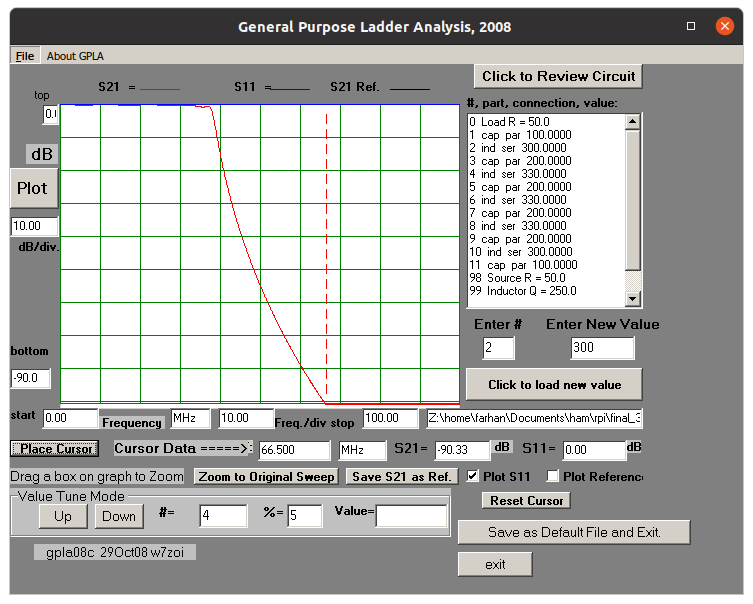
Figure 3
- Low quality capacitors and inductors. It is best to buy all the RF filter capacitors from a reputed online retailer like mouser.com or digikey.com. The only ones that are useful are the NP0 or the C0G variety. For inductors, the micrometal toroids are recommended.
- Insufficient shielding: Very often, the inductors are close to each other and the unintended coupling between them can heavily compromise the filter performance. Use a physical layout where the inductors are all in a line and oriented perpendicular to their neighbors. Shield the entire filter with copper sheets.
- Bad grounding: The filters have to be built over a large ground plane with short connections between the circuit components and the ground. Each component should be grounded separately. Longer traces or wires to the ground will add stray inductance that compromise the filters’ performance.
The Front-End
We use a passive FET front-end with +28 dBm IIP3 that is as simple to build as a diode mixer. It uses a single trifilar transformer and a low cost FET analog switch. Experimenters can also use a pair of switching mosfets like the BS170, etc. This front-end was first described a the KISS mixer by Chris Trask, N7ZWY in the paper Mixer Musings and the KISS Mixer. You can read this highly informative paper on https://www.mikrocontroller.net/attachment/146369/Mixer_Musings.pdf. Although Trask reported an astounding +40 dBm intercept point, he only measured it against a strongly terminated IF port. In our application, we directly drive it to (and during the transmit, from) a highly reactive crystal filter as a load which degrades the intercept point to some extent. The good news is that unlike a diode mixer, the local oscillator currents do not flow through the FET, making passive FETs more resilient to improper termination. Our measured intercept was at +28 dBm, with a loss of 4dB. The figure 4 shows the IMD with an input of -10 dBm / tone(disregard the marker of 1R, it is an artifact from a previous reading). The output is attenuated by 10 dB to prevent overloading of the spectrum analyzer. The IMD is barely recognizable at even this high power level.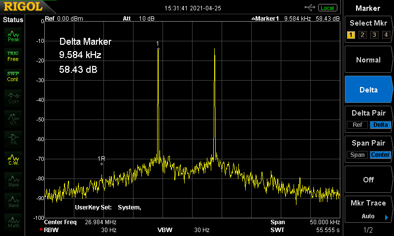
Figure 4
The Crystal Filter
Central to our radio is the 40 MHz crystal filter with a flat top and a very sharp upper side response. The filter begins as a Min-Loss Cohn filter with 2.2pF coupling capacitors and 2K termination impedance. We then, modify it by paralleling the ending crystals. This has the effect of doubling the motional capacitances and halving the motional inductance of the ending resonators, resulting in a relatively flat response.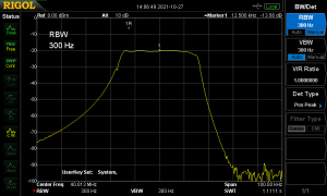 The figure 5 shows the response of the filter as measured on the sBitx PCB. Given that the coupling capacitors are just 2.2pf, the layout becomes critical. The center of the passband is at 40.013 MHz and there is a steep attenuation on the higher side, this is where we will position the second oscillator; somewhere close to 40.036 MHz.
The local oscillator(s)
We chose to go with the low cost Si5351Bx that is readily available, both as a chip and a module. It can simultaneously output three clocks at different frequencies. At a late stage in the design process, it was noticed that there is an internal ground bounce inside the chip that couples clock 0 output to clock 1 output. This leakage was less pronounced between clock 2 and clock 1. In the final design, we use clock 2 as the local oscillator to the front end. The clock 2 tunes from 40 MHz to 70 MHz, providing a coverage of 0 to 30 MHz. Using a slightly different front-end (for example, a diode mixer), it will be possible to extend the coverage to other VHF bands as well. The oscillator itself is capable of working in excess of 250 MHz. The clock 1 is used as the second oscillator, it can also be viewed as a BFO, except that the output of the diode mixer is not demodulated SSB. The clock 1 is about 25 KHz above the center of the filter’s passband, at 40.035 MHz. This results in a 25 KHz of RF signal being converted to the range of 11.5 KHz to 36.5 KHz, something that is easily handled by audio techniques and subsequently digitized using an inexpensive but high performance stereo audio codec. The Si5351 has better than average phase noise but not stellar. It can be considerably improved by using a low noise reference input instead of the in-built crystal oscillator. Hence, a low-cost Temperature Controlled Crystal Oscillator (TCXO) is used as the reference oscillator. This also eliminates the need for frequency calibration and alignment as the frequency is accurate enough for almost all amateur radio operations.The IF amplifier
The IF amplifier is a conventional feedback amplifier that uses BFR106. These are inexpensive and easily available transistors, though, alas only in SMD packaging. A strip of a hundred transistors will last you many projects. The measured OIP3 of these amplifiers is +30dBm. The noise figure is possibly 3dB (as per the datasheet). The homelab currently lacks a calibrated noise generator to measure this accurately. Until recently, the radio performance past the crystal filter was not very interesting as the dynamic range, etc. were all measured at 20 KHz spacing. The last quarter century has changed all this. The amateur operations are now clustered by modes within a few kilohertz of each other. All the FT8 work happens within 3 KHz bandwidth, most of the dxing is in the first 10 KHz of each band, the PSK31 happens in an equally narrow band etc. A local station running 100 watts of FT8 calling CQ can drown out all the DX even if you have a radio with 100 dB dynamic range, measured at the standard 20 KHz spacing. The dynamic range of the receiver has to be good enough all the way to the audio stages. Making feedback amplifiers bidirectional does seem to be a matter of simply putting them back to back. However, as the output of the active stage reaches levels exceeding -10 dbm, the base-emitter and base-collector diodes of the turned-off stage start to conduct and distort the signal. To isolate the turned off stage, three switching 2N7000 mosfets, the Q1, Q2 and Q5 are used as switches.Second Mixer and the ‘Audio’ Preamplifier
Our expectations are of 80dB in-channel dynamic range. At first, we used a KISS mixer similar to the one in the front-end, however it was found unnecessary as the IF amplifier and the following audio pre amplifier’s performance dominated and limited the dynamic range. Instead, we use the low cost BAT54S diode pairs as matched diodes in a conventional diode mixer. You could also use 1N4148s in its place. Note that we referred to the preamplifier as ‘Audio’. This is because the diode mixer output is at 24 KHz, not baseband audio. At this second IF, we can use standard audio techniques. The conventional audio preamplifier that follows a diode detector has compromised dynamic range. To address this issue, Wes Hayward, described an adaption of his now famous Termination Insensitive Amplifier to audio frequencies with far better performance. This is described at http://w7zoi.net/audio-fba.pdf. The preamp used in the sBitx follows the same architecture with very minor changes to accomodate what was available in the junkbox. This concludes the analog port of the receiver.The Analog Transmitter
The 24 Khz signal generated by the codec on the digital board is originally meant to drive 48 ohms earbuds. This is a good match to directly drive the diode mixer for upconversion to 40 MHz. However, as the codec is always on, it presents a potentially low impedance and at times noisy termination to the diode mixer in receive mode. Hence, it is isolated from the diode mixer on receive with yet another 2N7000 (at Q6)acting as an analog switch. The 40 MHz output is amplified by, and filtered in the crystal filter before being mixed down to the desired HF frequency in a reversal of the signal flow from the receive operation.The Power Amplifier

Figure 6
- The IRFZ24N gets so hot that the ordinary nylon bushing used to isolate the tab from the heatsink mounting screw can melt. Instead, we used a different scheme where a metal strip across the power transistors pressed them onto the heatsink with a mica washer in-between the transistors and the heatsink.
- We use a large heatsink that obviates the need for a noisy cooling fan. The same heatsink is also used to cool the LM338 that drops the 13.8v to 5V for the Raspberry Pi and the touch screen.
The Power Amplifier Transformer
The Digital Circuit
Before we discuss the details of the digital circuit, AN IMPORTANT CONCEPT: The left line input channel of the WM8731 is connected to the receiver preamplifier. The received signal samples at an Intermediate frequency of 24 KHz are captured by the codec’s left channel and transferred to the Raspberry Pi that does the SDR magic. The demodulated audio is then played back through the left earphone output. In effect, the left channel is used for receiver input and output. The right line input channel of the WM8731 is connected to a mic amplifier. The microphone input samples captured by the codec’s right channel are transferred to the Raspberry Pi that performs the SDR magic. The modulated 24 KHz signal is played through the right earphone output. The right channel’s input and output lines are used for transmitter input and output.
Figure 7
| Physical Pin on the Connector | Name | Purpose |
| 11,13,15 | GPIO0, GPIO2, GPIO3 | Input lines from the main tuning knob encoder and it’s push button |
| 19,21,23 | GPIO12, GPIO13, GPIO14 | input lines from the function knob encoder and its push button |
| 31, 33 | GPIO22, GPIO23 | Implements a separate bidirectional 2C bus to control the Si5351 (see text) |
| 7 | GPIO7 | Push to talk input |
| 29 | GPIO21 | DASH input line of the morse paddle, PTT is parallely used as the DOT line of the paddle |
| 16 | GPIO4 | T/R output line |
| 18,22,24,26 | GPIO5, GPIO6, GPIO10, GPIO11 | Output lines to select 1 of the 4 low pass tx filters |
| 32,36 | GPIO26, GPIO27 | Extra I/O lines |
The Software
The sBitx software is especially written to be understandable, hackable and extensible. It is also constantly being updated. You can grab the latest version from https://github.com/afarhan/sbitx. There are accompanying notes in install.txt if you are doing a fresh install. The core SDR routines rx_process() and tx_process() are really simple and easy to understand. We will examine them in a broad way but the best way is to just read the source code and ask questions about it in the bitx20 forum at https://groups.io/g/bitx20 Unlike the Arduino/Teensy programming, the sBitx works on a very powerful, quad CPU ARM core with graphics accelerator, etc. It uses all the power of such a powerful operating system to build a simple and straightforward code base where readability is preferred over speed and optimization.This is a Convolution SDR, WHAT!
Imagine you have a direct conversion radio with an audio bandwidth of just 1 Hz. You have an extraordinarily long piece of paper to write things on and a magical junkbox full of VFOs that can be set to any frequency and starting phase. You tune across the band, stopping at every 1 Hz and noting the DC signal’s strength and phase. You can now use this list of frequencies and their strength and phase to plot the spectrum on a piece of paper bins drawn in them. This is how conventional analogue spectrum analyzers work. To use the correct jargon, this process has converted the signal from time-domain into frequency-domain. We will also refer to each entry that you make in the list as a ‘bin’. Let’s reverse this experiment. You have your bins of frequencies and the amplitude/phase at each frequency. And you have a magical junk-box in which you have an unlimited supply of VFOs that you can set to any frequency and starting position (phase). To generate the entire band’s signal back, you take one VFO at a time, set the exact frequency and phase as per your list and switch them on at once. Viola! you have lit up the entire band of signals recreated as it was in the written down list! Rather, you have converted the frequency domain signals back to the time domain. In the above thought experiment, note that not just the CW, every signal can be written down as a series of measurements of amplitude and phase at different frequencies and reconstructed back using a series of frequency generators. The above process can be done, mathematically and hence on a computer as well. How does this help us in generating or receiving, let’s say an SSB signal? Now, let’s imagine that there is an upper side band signal exactly at 14.150 MHz. We started measuring the signal from 0 Hz and continued until 14.200 MHz, we have effectively filled up 14,200,000 bins with information, in frequency domain. We took 14,200,000 precise measurements of how much the amplitude and phase was at every 1 Hz step. You will see the reading values starting with frequency 14,150,000 Hz going up depending upon the instantaneous voice modulation of the incoming signal. By the time you reach 14,153,000 Hz, the signal strength would have dropped as the SSB occupies less than 3000 Hz bandwidth, you nevertheless continue your assigned job and reach 14,200,000 Hz. Stop, massage your hand and have coffee while staring down at your clipboard. Now, we take a new clipboard and starting copying the bins into it but we start at the bin of 14150000 Hz and write the value of that bin as bin 0 on the new clipboard, we move to the bin at 14150001 Hz and write that down as bin 2 and so on. By the time we have written 50,000th bin on the new list, we have reached the end of the old list at 14,200,000 Hz. We continue to fill the rest of the bins in the new list from bin 0 of the old list and continue all the way up to the list’s bin of 140,149,999. The new list has all the bins and readings of the old list except that is is rotated around such that the first element in the new list corresponds to the 14,150,000th element of the old list. Next, we will set about doing some slash and burn (also called filtering). We will zero all the bins except the first 3000 that correspond to our signal. This eliminates any signals apart from the specific 3 KHz slice that we are interested in. Also note that we have eliminated the other sideband. The lower sideband image of the signal would have been in the bins of the frequencies from 14147000 Hz to 14150000 Hz and along with all the other bins, those were turned to zero as well. Now, we take this list of frequencies and set about our VFOs to correspond to each of them and power them up! Your SSB signal is now translated to audio, the lower sideband is eliminated, the rest of the signals are filtered away. Let’s see how this is practically implemented in sBitx.Receiving single sideband, Convolution!
There will be a number of implementational details that any working code has that distracts from its core work, on the other hand, the sBitx core SDR is written to be understandable and hackable. So, we will skip a few things in the code on the first pass. Right now, just remember two things: 1. The sbitx handles a block of 1024 samples at a time. As both channels (left and right) are running all the time, the function rx_process() is called with the next set of received signals from the receiver circuitry as well as the microphone samples. We just ignore the microphone samples while running the receiver code. 2. The frequency of any signal can only be known if it is a continuous sine wave. When we start and stop recording any signal there is an abrupt beginning and an abrupt end to it that confuses any mathematical operation. To smoothen this out, we process not 1024 but 2048 samples at a time. The first of these 1024 were what we received in the earlier call to the rx_process() to this we add the newly arrived 1024 and run the FFT over the combined lot of 2048 samples. This way the distortion from the abrupt beginning happens on the samples of the first 1024 samples. We are not bothered about the distortion in those first 1024 samples because they have already been processed earlier. We simply discard them. This technique is called overlap-and-discard. Now, we can read the code and understand it quickly.void rx_process(int32_t *input_rx, int32_t *input_mic,
int32_t *output_speaker, int32_t *output_tx, int n_samples)
{
int i, j = 0;
double i_sample, q_sample;
//STEP 1: first add the previous M samples to
for (i = 0; i < MAX_BINS/2; i++)
fft_in[i] = fft_m[i];
//STEP 2: then add the new set of samples
int m = 0;
for (i= MAX_BINS/2; i < MAX_BINS; i++){
i_sample = (1.0 *input_rx[j])/200000000.0;
q_sample = 0;
j++;
__real__ fft_m[m] = i_sample;
__imag__ fft_m[m] = q_sample;
__real__ fft_in[i] = i_sample;
__imag__ fft_in[i] = q_sample;
m++;
}
// STEP 3: convert the time domain samples to frequency domain
fftw_execute(plan_fwd);
struct rx *r = rx_list;
//STEP 4: we rotate the bins around by r-tuned_bin
for (i = 0; i < MAX_BINS; i++){
int b = i + r->tuned_bin;
if (b >= MAX_BINS)
b = b - MAX_BINS;
if (b < 0)
b = b + MAX_BINS;
r->fft_freq[i] = fft_out[b];
}
// STEP 5:zero out the other sideband
if (r->mode == MODE_LSB || r->mode == MODE_CWR)
for (i = 0; i < MAX_BINS/2; i++){
__real__ r->fft_freq[i] = 0;
__imag__ r->fft_freq[i] = 0;
}
else
for (i = MAX_BINS/2; i < MAX_BINS; i++){
__real__ r->fft_freq[i] = 0;
__imag__ r->fft_freq[i] = 0;
}
// STEP 6: apply the filter to the signal,
for (i = 0; i < MAX_BINS; i++)
r->fft_freq[i] *= r->filter->fir_coeff[i];
//STEP 7: convert back to time domain
fftw_execute(r->plan_rev);
//STEP 8 : AGC
agc2(r);
//STEP 9: send the output back to where it needs to go
int is_digital = 0;
if (rx_list->output == 0)
for (i= 0; i < MAX_BINS/2; i++){
int32_t sample;
sample = cimag(r->fft_time[i+(MAX_BINS/2)]);
output_speaker[i] = sample;
output_tx[i] = 0;
}
}
Open the file at https://github.com/afarhan/sbitx/blob/main/sbitx.c and scroll down to the function that says rx_process(). It might even help to take a print out of just this section to read along with the explanation here.
We start with Step 1 of first copying 1024 samples of the previously received samples into the array fft_in[] and in Step2 append that with samples passed from the codec as input_rx).
Now in Step 3, we simply called the excellent fftw library to convert all the samples to frequency domain. No, we didn’t have to write that code ourselves. the fft_execute() function sets the frequency domain data in the fft_out[] array.
The variable tuned_bin is the bin of the signal that we are interested in listening to.
In step 4, we fil another array called the fft_freq[] with the data from the fft_out[] such that the fft_freq[0] has the starting at the tuned_bin.
In step 5, we zero the other sideband.
In step 6, we apply filtering. This is interesting and unusually simple. Radio amateurs are used to looking at filter graphs where the frequency is on the x axis and the response is on the y axis. We have plotted the crystal filter and the low pass filter shapes above in this paper in a similar way.
For filtering in frequency domain, we make a filter shape out of a set of frequency bins. We set to zero all the frequencies that we don’t want to pass and ‘1’ for all the frequencies that we wish to let through. Making a filter this way is a bit crude because there are edge frequencies between two bins that can introduce distortion in the filtered output. Hence, we apply a windowing function to smoothen out the filter edges, that source code is in https://github.com/afarhan/sbitx/blob/main/fft_filter.c . It was borrowed from Phil Karn’s excellent radio project at https://github.com/ka9q.
Each time the filtering setting is changed, we generated a new filter as set of frequency domain bin values.
Applying the filter is just a matter of multiplying the filter bins with the frequency domain signal bins. It is beautifully simple.
Our signals are now in the frequency domain, they are shifted to the baseband, filtering has been applied.
In step 7, we convert the signal back to time-domain so that they can be played by the codec.
In step 8, the audio’s amplitude is normalized in the function agc2() so that a strong signal doesn’t blow your eardrums. We will not cover it here except to say that the agc2 looks for the maximum amplitude in the block of samples; if it exceeds the previous maximum, the gain is set to bring it down to a set level. The gain remains ‘hanging’ even after the strong signal disappears while agc_loop counts down to zero. The agc response can be slow or fast depending upon the value set in the agc_speed variable.
That’s all there is to it.
Transmitting is just the reverse
The transmission process happens in tx_process() function. It is very similar to the rx_process() though in reverse. The block of baseband audio samples previously received from the microphone and the currently received samples are all assembled into a bin of fft_in[] array, converted to frequency domain with fftw_execute() and the resulting frequency domain signal is filtered to restrict the audio to permissible bandwidth. The bins corresponding to the opposite sideband are set to zero. The bins are now rotated to bring the signal to the desired frequency and converted back to time-domain with another called to fftw_excute(). Optionally, on USB and LSB, compression is applied to increase the average transmitted power and increase the intelligibility of the signal.The Modems (aka Waveforms)
The power of sBitx comes from being able to handle many of the digital modulation methods transparently. The sBitx uses the excellent fldigi for all the keyboard to keyboard modes (including CW decoding) and Karlis Goba’s FT8 library for FT8 (available at https://github.com/kgoba). Rather than a line by line exposition of the way the code works, we will provide an overview so that those interested in adding more modes can use this as a guide. There are many kinds of modems that are in vogue. Some process all the samples together in a bunch like the WSJT-X suite of protocols. Others like PSK31, RTTY or even CW (it is a digital mode!) are handled one sample at a time. The external modems are interfaced with the main routines like the rx_process() and tx_process() by reading and writing from a second virtual sound card. We create the virtual sound card by running a linux utility called snd-aloop. It creates three virtual sound cards and we use two of them. These virtual sound cards are named plughw1, plughw2, plughw3. Each one of them further has two subdevices as 0 and 1. These are unfortunate names handed out by the Linux operating system. Along with playing the audio to the speaker, the sbitx also plays to the virtual device plughw:1,0. During transmission, instead of reading from the microphone, the samples are read from plughw:2,1. This is done transparently in the sbitx_sound.c. Accordingly, the modem software (like Fldigi) should set their record device to plughw:1,1 and play device to plughw:2,0. The interface to the modems is through a simple set of functions implemented in modem.c. The important one is modem_poll(). It is called a few times every second. It monitors any change in the modes, transition from transmit to receive etc. The other is modem_get_sample() which is used to generate the required waveforms, one sample at a time. This may be studied for how CW is generated from keystrokes or the paddle. The excellent suite of modems in fldigi, written by Dave W1HKG and his team is integrated with sBitx as slave. The sBitx controls the fldigi using its XML-RPC interface : changing modes, reading decoded text or sending more text from the keyboard. The audio samples flow to and from using the virtual audio cable as mentioned above. For FT8, we didn’t use the WSJT-X, instead we used the command line encoder and decoder written by Karlis Goba. The samples are collected in subsequent calls to modem_rx() and on every 15th second, it is written into a file and decoded by calls to the command line utility ft8_decode, the text output is displayed on the radio’s console. For transmitting FT8, the text is submitted to gen_ft8 which produces audio samples. These are picked up every 15th second and transmitted.The User Interface
- The user interface of the radio has to satisfy many conditions:
- 1. It has to be equally usable from the front-panel with the Tuning and Function encoders and touch interface or the keyboard.
- 2. The user interface is delinked from the core sdr and a wholly different user interface can be substituted. The core sdr receives commands as text strings through sdr_request(). Any alternate program can generate these instead of the sbitx_gtk.c that is currently available.
Simple and adaptable, portable
The User interface has to be quickly programmable by experimenters who just want to get it done rather than study how GUIs are written. The current GUI takes minimal help of GTK and using primitives to : a) draw lines, write text and fill rectangles. b) Be notified of mouse events and keystrokes From these basic routines, we build our own user interface that consists of a single user interface element described in the struct field. The struct field, whenever it is updated, in turn automatically calls the functions to be executed with the new value or actions. The struct field member cmd is the actual text command to be executed when the field is changed or touched. Most of these commands are directly passed to the core sdr. Some of the commands that implement functional on top of the core SDR (like macros, etc.) have an asterisk ‘*’ in the beginning of their command name. Some fields are special (like the waterfall) and they have to be drawn differently. For those cases, the default handling of their corresponding struct field is over-ridden by providing setting the fn member to a function that will handle the events and provide a custom drawing routine.Text friendly
The commands entered from the keyboard are executed by the function cmd_exec(). It should be fairly easy to port it to other operating systems like Microsoft Windows or the Macintosh. The base system works on text commands that can even be passed through a primitive telnet like interface. This makes it easy to adapt this to smaller displays or even an eyes-free implementation for the visually challenged. On the other hand it is also easy to build a remote, web-based front-end for the radio. It is hoped that these features will come in very soon.Read The Fine Manual!
The list of features and commands is ever growing. It is best to periodically download the latest The Operating Manualversion from https://docs.google.com/document/d/1fQXQoQSHD_YDnZYGjL6JCdR8Klfg4KE-FuN-5BE1OSQ/edit?usp=sharingAlignment
As it is all in the software and the frequency is determined by a TCXO, there is very litte alignment needed. You just have to set the bias for the driver and the power amplifier.- Set the PA and drive presets to fully counter-clockwise. Add Ampere meter (your VOM should have a 10A range) to the power supply to monitor the radio’s current.
- Switch to either LSB or USB and press the PTT without speaking (silence!).
- Now, carefully turn the DRIVE bias preset clockwise until the current starts to climb, set it to an increase of 200 mA (100mA per transistor).
- Next, carefully turn up the PA bias preset clockwise until the current starts to climb, set ti an increase of a further 200 mA.
Hacking and modifying the sBitx
Here is how you can get started with experimenting with the sBitx software. We will see how the sBITX is laid out and how to quickly start changing things. The latest source code can always be found on https://github.com/afarhan/sbitx.Quick Start
If you received the sBitx as a ready-built system, you will find the source code in /home/pi/sbitx directory. To build the system you execute the batch file build as thus: cd /home/pi/sbitx (to change to sbitx directory) To build the radio, ./build sbitx (remember the dot before the slash) To start the radio, ./sbitxHow it is laid out
The sBitx is all about being able to find your way in the weirdness of software defined radios, hence every attempt is made to keep it simple and quick to understand. We assume a minimum familiarity with the C language and being able to use a text editor. The idea is to make it easy to carry the system from platform to platform. The big idea of sBitx is that is NOT a phasing SDR. It is a superhet with first IF at 40 MHz that is downconverted to a second IF of 24 KHz. The 24 KHz IF is digitized through a high speed, low-noise audio codec. In this specific case, it is the WM8731. In broad strokes:- The core SDR is on sbitx.c and it has no user interface around it. It gets samples from the audio system and writes them back to the audio system. It accepts commands to change modes, volume, etc., as text strings when the user interface calls sdr_request(). This is where the samples from the mic arrive, get processed and sent to the radio (when it is transmitting) or they arrive from the radio, get processed and sent to the speaker (when it is receiving). These two routines are rx_process() and tx_process().
- We use convolution method to do the actual modulation/demodulation. It is much simpler to understand. It is best explained by Gerlad Youngblood, K5SDR in his seminal papers called A Software Defined Radio for the Masses. Read them here and here. Better yet, print them out and read and re-read them until you understand the concept. A few tricky details like save-and-overlap convolution or wrap-around with imaginary frequencies are not required knowledge to hack. If you insist, read them on https://www.dspguide.com/.
- We do our own GUI. The regular GUIs of Linux/Mac/Windows don’t quite work for radios. Each is pretty complicated as well. We also imagine that in the future someone might want to port the sBitx to an embedded system. Besides, most of us have no time to learn intricacies of GUI programming. Instead, we took the basic ability to draw lines, rectangles and text and built our own simple user interface. All that is in sbitx_gtk.c.
- It is written in simple C language. in a particular style of using all smalls as the names of functions and variables and it hasunderscore between the words (do_cmd() instead of doCmd or DoCmd). The lines are formatted such that they can fit into the 7 inch Raspberry Pi screen. We use the opening brace on the same line as the if or while statement to make efficient use of the 7 inch display of the sBitx.
- Stick to 2 spaces per tab, braces in the same line as the if or while statement. This is not religion but utility. The compact display of the sBitx can’t show too many lines. We follow the Linux coding style.
The Sound System
The details of sound sytem are all hidden in sbitx_sound.c. There are a few things to remember- The sampling rate is fixed at 96,000 samples per second. Each sample read or written to the hardware is a signed 32-bit integer. The audio hardware works in full duplex at all times.
- The digital IF is centered on 24 KHz, staritng from 12.5 KHz to 37.5 KHz.
- The left channel is dedicated to receive. It gets its samples from the demodulator (Actually, the downconverter that moves the 40 MHz IF to 24 KHz, which is kind of “audio” range, handled by the audio codecs). After processing it writes the samples back to the speaker.
- The right channel is dedicated to transmit. It gets its samples from the mic, processes them and writes the transmit signal samples to the right channel.
The GUI
The GUI and other platform specific details are implemented in sbitx_gtk.c. The GUI is build around a single structure called the field. This represents a single element on the screen (like the waterfall or a button)struct field {
char *cmd;
int (*fn)(struct field *f, cairo_t *gfx, int event);
int x, y, width, height;
char label[30];
int label_width;
char value[MAX_FIELD_LENGTH];
char value_type; //NUMBER, SELECTION, TEXT, TOGGLE, BUTTON
int font_index; //refers to font_style table
char selection[1000];
int min, max, step;
};
The field cmd holds the text string that is to be sent as the command to the core sbitx. Many functions are not core to the sbitx. For instance, RIT (Receiver incremental tuning) is implemented as user-level feature that changes the core sbitx frequency between receive/transmit. The commands that are not to be passed to the core sdr are prefixed with a ‘#‘.
There are a few kinds of controls defined. All of them are in square boxes that can be easily touched by stubby fingers. These are the different kinds of controls
- Button: These have no ‘value’ just a label (Ex: Close)
- Selection: These can have one the selection of texts given in the selection field. All values are text strings, separated by forward slash’/’. (Ex: Mode selector)
- Toggle: Essentially a selection with two values, when you click on it, it changes (like VFO A/B, RIT On/Off, etc.)
- Number: Like a volume control or gain control. It can take any value between min, max in jumps of step.
- List: This is takes a long text that is wrapped around or broken with new line characters. The text scrolls past.
- Text: You can enter text in these fields
Before you make any changes
Save the current snapshot of the source code using the git like this:git commit -a -m “Saving the original, just in case, hehe”
This command commits (saves) the current snapshot. The -a means all of it, -m says, a message is to remember what the commit is all about. To see the history of all the previous commitsgit log
This lists the last few commits, Each commit is listed with the comment as well as a unique checksum. To revert to a previous commit,git checkout [checksum] (You can specify just the first few letters of the checksum)
This is the shortest introduction to git, learn more from the Internet.Debugging
We use the standard linux debugger gdb. You can read all about it in the manual (Run : man gdb). However, here is a quick start for those who don’t read manuals. Start it like this:gdb sbitx
To run the sbitx, type the command(gdb) r (Run the program)
To set a break-point(gdb) b sbitx.c:100 (Sets breakpoint when execution reaches a particular line)
(gdb) b rx_process (Sets breakpoin when the execution reaches the function rx_process)
To see a variable(gdb) p last_mouse_x (Prints the value of the variable)
(gdb) p *f (Prints the structure/variable pointed by f)
To step inside the function on the current line(gdb) s
To step over the current line to the next(gdb) n
To resume execution of the sbitx after watching/stepping past a break-point(gdb) c
To see the stack of called functions (back trace)(gdb) bt
To get out of the debugger(gdb) q
Learning more
There are some really amazing resources online to help you understand how SDRs work and in particular how the sBitx works. Here is a starting list : K5SDR’s seminal papers in QEX. These are avaiable from https://sites.google.com/site/thesdrinstitute/A-Software-Defined-Radio-for-the-Masses Bob Larkin’s QST papers describing the DSP-10 Transceiver, the inspiration for sBitx. http://www.arrl.org/software-defined-radio Phil Karn’s SDR receiver project from which much of the filtering code has been borrowed. https://github.com/ka9q/ka9q-radio Wes Hayward, Rick Campbell and Bob Larkin’s book Experimental Methods in RF Design. Now out of print, grab a copy. It has the most radio ham friendly introduction to DSP and SDRs. Steven Smith’s amazingly direct and in-depth treatment of DSP stuff https://www.dspguide.com/ Wes Hayward’s website for more details on the high dynamic range AF pre-amp and other filter related papers. https://w7zoi.netAdapting to your own circuits
It is hoped that this work will encourage others to adapt this software to more radios. Three things need to be changed:- Route the digital I/O lines that flip between tx/rx, change the tx filters and sense the PTT and keyer paddle to your radio’s circuit.
- In sbitx.c, change the routine that sets the local oscillator to your radio’s way of doing it.
- Rewrite the audio loop in sbitx_sound.c to suit the audio hardware that you are using.
Leave a Reply