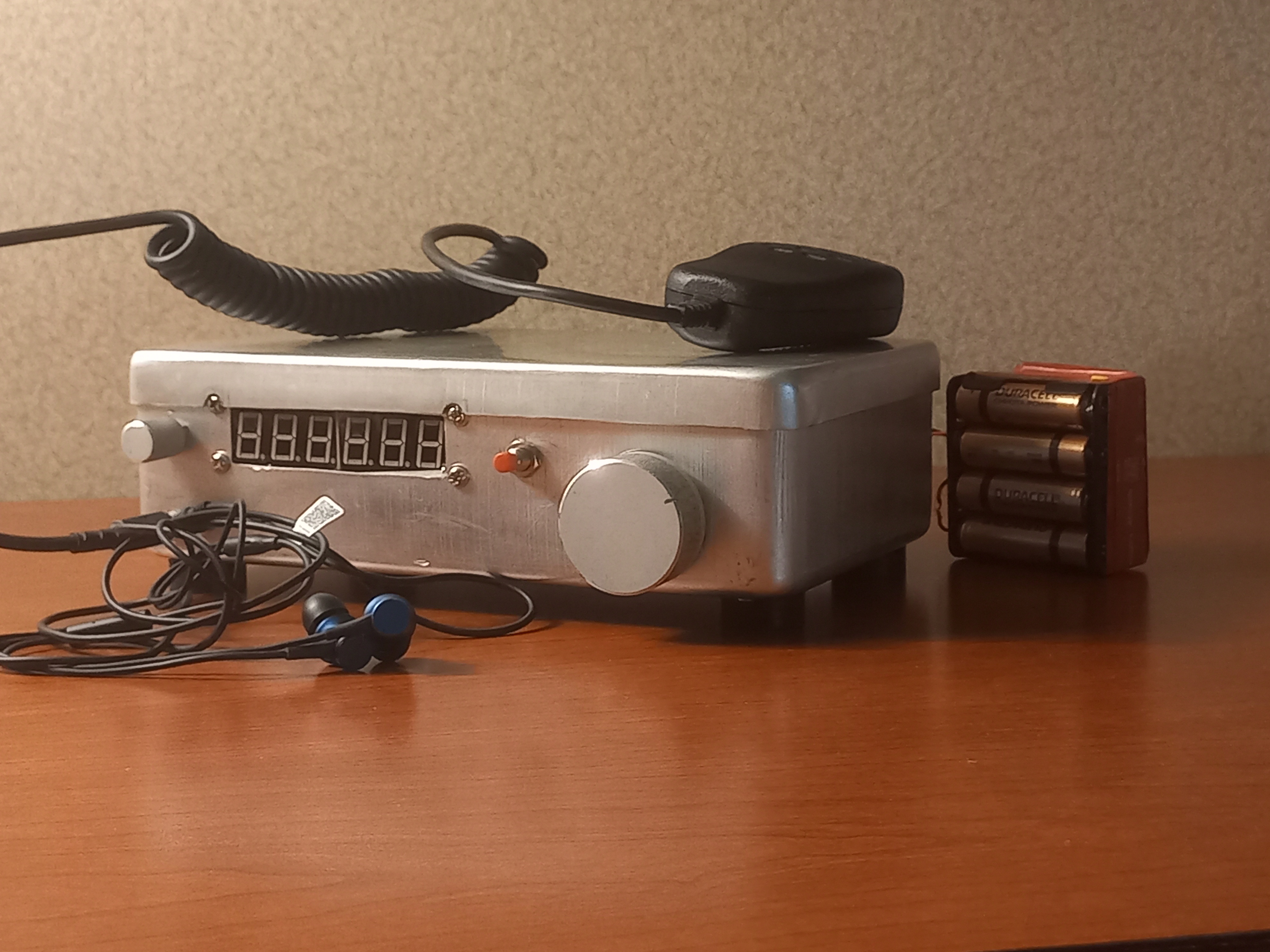
Daylight Again – An all Analog Radio
 What’s all this?
In 10 seconds,
What’s all this?
In 10 seconds,
- A high performance, 7MHz, 5 watt SSB rig
- Draws just 24 mA of current
- 90 dB dynamic range, 80 dB close-in dynamic range
- 3D printed rock stable, slow tuning PTO with zero backlash.
- 3D printed toroids
- You have all the parts in the junk box or you can buy them tonight at the vendor night.
- Very stable, slow tuning VFO with no backlash
- Costs less than 20 dollars to build, even in new parts.
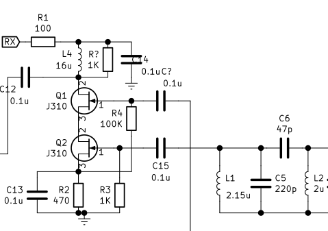
The Circuit Diagram

Full Circuit Diagram
Isn’t analog radio an anachronism? Are we just being nostalgic? What’s wrong with the Si5351?
Last year, when we had to isolate ourselves for a week, I managed to grab some components, an Antuino (the RF lab in the box), some basic tools and set about making a slightly souped up version of Roy Lewallen’s Optimized Transceiver from our room. The experience of a well designed analog rig was truly enlightening. There were no spurs, the audio was crystal clear and with presence. When David NM0S and I were discussing this year’s FDIM, I suggested that we do a return to analog radios and he jumped at it! So here we are, talking analog radios in 2022. Here is the memo : The analog never died. The world is analog all the way, until you descend into Quantum madness. The antennas are analog, Maxwell died a content, analog man. Our radios, ultimately, are analog machines and we are all analog beasts too. Amateur Radio technology has evolved into the digital domain. However, it has only made it easier for us to do analog with computers to simulate and print our circuits. So, it’s time to bid good bye to our Arduinos and Raspberry Pis and build an Analog Radio for ourselves. So let’s see what we can achieve in hindsight, a return to our native land and a rethink of our approaches. The radio is called Daylight Again, a nod to being back at the FDIM in 2022 after a gap of two years. It is named after the Crosby, Stills, Nash and Young’s song that had been humming all the time while put this radio together, emerging after 2 years of lockdown. This radio that took two days to come together, no actually two years! That’s: parts of it got built and stowed away, thoughts were struck in the shower, questions popped up during early morning cycle rides and notes and circuits were scribbled in the notebook. I must take the first of many diversion here: I hope you all maintain a notebook. Write down the date and whatever you thought or did on the bench and the result. Nothing is trivial enough to leave out. Wisdom comes to those who write notes. I started to build this on Saturday the 14th May and I checked into the local SSB net on Monday morning, the 16th May 2022. Back to the radio. What can an analog radio do that will appeal to us homebrewers?-
- Simple to build (?) This is a myth as this paper will demonstrate. It may be easy to duplicate a design from the QRP Journal or the Sprat, but to design a radio that is stable, sensitive, selective and sounds sweet on air is not trivial. It needs thinking and revisiting our assumptions and habits (like the diode mixers).
- Low power: The radio draws just 24 mAYes, an analog radio can be really really lean. Low power is not just a show-off. It has some real purpose. One can work for weeks from a single pack of AA cells. Working your rig off a battery pack eliminates a large species of noise and spurs; As things stay cool inside, the VFO drift is much lower and one could carry the rig on a cycle!
- Low noise VFO.What’s the big deal here? All local oscillators are the same, isn’t it? Not really. Consider each VFO to be an AM transmitter that splatters around the carrier. As the VFO splatter mixes with an incoming signal that is strong and yet off your receiver frequency, to the listener it appears as if the signal has splatter. Actually, the signal would be entirely clean, it is your own local oscillator’s splatter that you are hearing.
- Having clean VFO is the most important way of increasing the dynamic range of your radio. A free running JEFT VFO that has sufficient power and a good Q components, will be unmatched by any synthesized or direct sampling radios. The math is all on the side of the free running VFO. We are talking -150 db/Hz at 10 KHz spacing, by comparison the Si5351 is -125 db/Hz, it is 300 times worse.
- Stability of 2 Hz/15 second. Can it decode FT8? Actually yes, we have had regular decodes after 15 minutes of warm up. It stays stable enough for CW and SSB. WSJT-X suite is the main challenge. We need a stability of better than 2 Hz/15 second period for the WSJT-X suit to work. We do this by keeping the operating frequency of the VFO low, eliminating heat around the VFO and using sturdy but ugly, short and stiff point to point wiring.
- Dynamic Range of 90 dB and close-in range of 80 dB. The real, tough, beef eating hams don’t care for dynamic range, we operate! Right? Wrong. The bands have changed. Signals tend to cluster within narrow pockets. All the QRPers hang out on 7040, the PSK gang is over at 7060, the FT8 kiddies are parked at 7074. The local charminar net at 7080, long after it is closed, has the hanger-ons late into the noon. We need radios where we can clearly make out a CW pileup where you can hear 20 different stations at once.The 90 dB is actually a very good number. The gains beyond this are marginal. Unless you are operating with full power stations within close neighbourhood on the same band as you, 80 dB of close-in dynamic range is enough to win you CW sweepstakes. Ask Rob Sherwood (https://www.youtube.com/watch?v=GNh0wP9PlsM).
- Why SSB? Just because it is a more complex thing to build. It is easier to add CW to an SSB rig rather than add SSB to a CW rig. The amplifiers need to be linear, sideband needs to be suppressed etc. We may add CW to this rig later.
- Undo the Lore.We homebrewers tend to stick to the beaten path. We build exactly the same radios over and over again. When was the last time you didn’t use a diode mixer? Or build radios that didn’t use 50 ohms interconnect? It is about time.
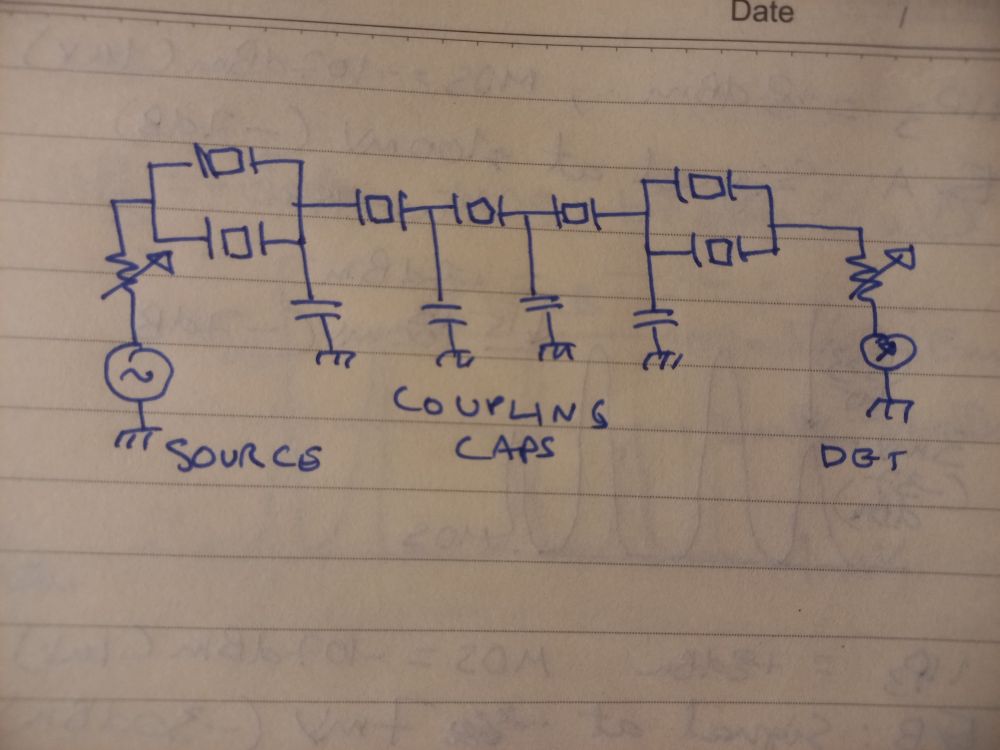
The Cascode Mixer
 Remember the 70s when Doug, W1FB built those radios with 40673 dual-gate MOSFETs? Well, they are back! It is 2022 and they are exhibiting good dynamic range, we are rebooting the old heros.
The dual-gate MOSFETs are, surprisingly enough, still being manufactured. Mouser lists tens of thousands of them, they are cheap but available only as SMD parts. However, you can build a virtual dual-gate FET from two JFETs, it works all the same. A bag of 100 J310s is still sold for a few dollars at Dan’s (. With careful design, a cascode can provide us with +8dbm of input intercept and a gain of 10 db. This might not seem much to most but it is.
This is more than respectable, it is downright awesome. Here is why: The cascode mixer with +8 dBm of Input intercept(IIP3) and with 10 dB gain over it has an OIP3 (output intercept) a huge +18 dbm (calculated as IIP3 + gain).
In comparison, the diode mixer with +15dbm input intercept has a loss of 7 db and noise figure of 7db (actually the loss is the noise figure). Thus a diode mixer’s output intercept is +8 dBm (again calculated as IIP3 + gain, that is negative loss in this case) as compared to +18 dBm of the JFET cascode.
There are several striking things about this mixer:
Remember the 70s when Doug, W1FB built those radios with 40673 dual-gate MOSFETs? Well, they are back! It is 2022 and they are exhibiting good dynamic range, we are rebooting the old heros.
The dual-gate MOSFETs are, surprisingly enough, still being manufactured. Mouser lists tens of thousands of them, they are cheap but available only as SMD parts. However, you can build a virtual dual-gate FET from two JFETs, it works all the same. A bag of 100 J310s is still sold for a few dollars at Dan’s (. With careful design, a cascode can provide us with +8dbm of input intercept and a gain of 10 db. This might not seem much to most but it is.
This is more than respectable, it is downright awesome. Here is why: The cascode mixer with +8 dBm of Input intercept(IIP3) and with 10 dB gain over it has an OIP3 (output intercept) a huge +18 dbm (calculated as IIP3 + gain).
In comparison, the diode mixer with +15dbm input intercept has a loss of 7 db and noise figure of 7db (actually the loss is the noise figure). Thus a diode mixer’s output intercept is +8 dBm (again calculated as IIP3 + gain, that is negative loss in this case) as compared to +18 dBm of the JFET cascode.
There are several striking things about this mixer:
-
-
- Take very little VFO power The oscillator injection on Q1 is to the gate, it takes zero power of local oscillator injection (the current never flows into the JFET gate). This results in the VFO running cooler and with less drift and less current consumption!
- Needs no post-mix amplifier This mixer is insensitive to termination and it is unidirectional. The signals will not flow back from the drain to the source. You don’t need to follow this up with a post mixer amplifier that will draw even higher current. Conventionally, a diode mixer needs 5 milliwatts of local oscillator, which means that the oscillator itself must draw about 100 milliwatts to produce it and the diode mixers invariably need a post mix amplifier with about 20 ma of standing current, which, at 12 v will amount to 12 x0.02 = 240 milliwatts of power. In effect, together, the diode mixer and its post-mixer amplifier up the receive budget by 340 milliwatts. People of the GQRP and QRPARCI clubs have attempted DXCC with those power levels!
- You can pick your own working impedance. To get upto 10 dB of gain, you will need to set the input and the output impedances to around 2000 ohms. However, at lower the impedance and the gain will decrease but the other mixer parameters will remain as they are! You can put this into LTSpice and smoke it. This makes the job of matching input to an RF band pass filter or the output to a crystal filter very easy.
- The output has an unsuppressed local oscillator. There is no balance, at least, in this simple design. We can add balance by using another similar mixer in push-pull configuration though as a receiver front-end mixer, our purpose is served without needing to suppress the local oscillator. The RF front-end can directly drive the crystal filter. However, the cascode mixer is unsuitable as a transmit mixer due to this oscillator leakage and we will use an NE612 for that as discussed later.
- Noise figure is 4 dB. This is really sensitive. You can build high grade VHF/UHF mixers with this sensitivity.
- Input Intercept of +8 dBm This needs some illustration. +8 dBm is about 7 milliwatts of power. When you overload the mixer with an unwanted signal of 7 milliwatts, the distortion produces unwanted signals that appear to be 7 milliwatts too, it is where the distortion is equal to the signal itself. This is a theoretical limit.
-
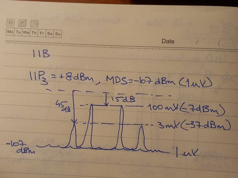
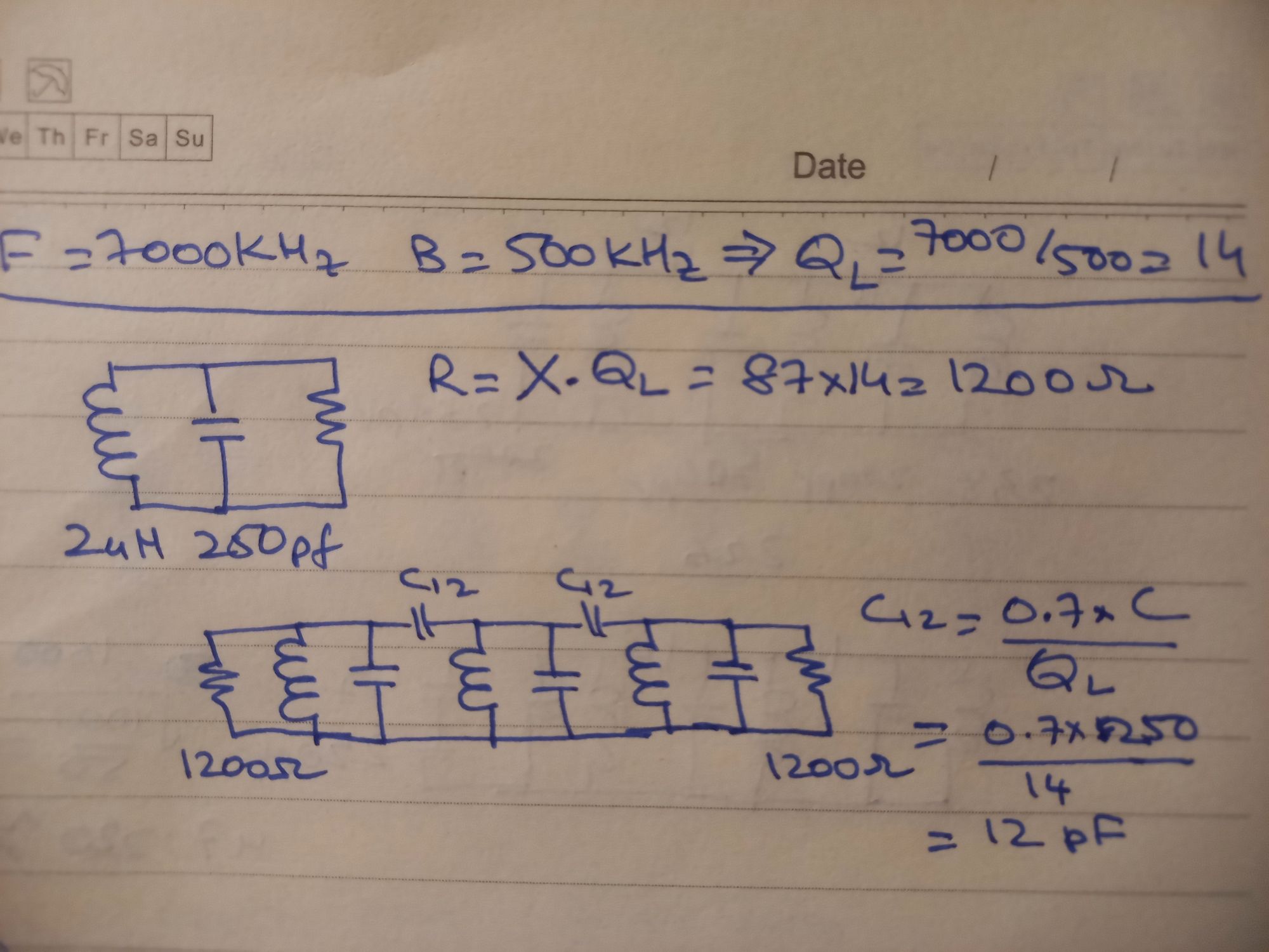
Notbook calculations of the IMD
Controlled Gain, Block by Block
Our craft consists of stringing together filters, amplifiers, mixers and oscillators together. One wonders : Is there a point in putting an IF amplifier at all? Should I add an RF amplifier? Is it better to replace the diode mixer with an NE612? It is confusing all the way!
NR60, a homebrew design of the 1980s that wasn’t optimized for distortion
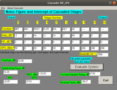 It works simply by filling in a table of columns, each column represents one stage of either a transmitter or a receiver. For each stage you specify the noise figure, gain and output intercept (OIP3). Most RF chips, or circuit blocks do specify their performance in these three critical parameters.
[A Tip: In passive circuit blocks like the filters or diode mixers, the noise figure is the same as the loss. So, if a bandpass filter has a loss of 2dB, consider that to be its noise figure as well. For passive filters you can assume the OIP3 intercept to be +50 dBm]
I wrote a web version of the same calculator. Once you have populated all the stages, you press the button and it gives you the results. It is available on https://www.vu2ese.com/index.php/2021/05/17/cascade-calculator/.
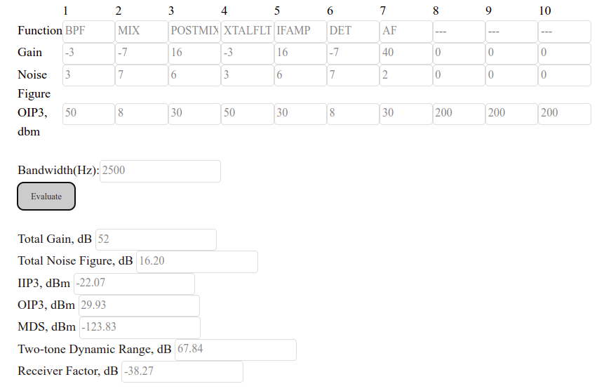
Here is a traditional superhet built the traditional way. Let’s examine it:
It works simply by filling in a table of columns, each column represents one stage of either a transmitter or a receiver. For each stage you specify the noise figure, gain and output intercept (OIP3). Most RF chips, or circuit blocks do specify their performance in these three critical parameters.
[A Tip: In passive circuit blocks like the filters or diode mixers, the noise figure is the same as the loss. So, if a bandpass filter has a loss of 2dB, consider that to be its noise figure as well. For passive filters you can assume the OIP3 intercept to be +50 dBm]
I wrote a web version of the same calculator. Once you have populated all the stages, you press the button and it gives you the results. It is available on https://www.vu2ese.com/index.php/2021/05/17/cascade-calculator/.
Here is a traditional superhet built the traditional way. Let’s examine it:
-
-
- We have a band pass filter in the front-end, followed by a diode ring mixer that has about 7 db loss, the diode mixer needs a post-mix amplifier to terminate it properly,
- A 2N3904 biased at 20 mA would provide us with a strong post-mix amplifier with +30 dBm OIP3,16 dB gain and 6 dB noise figure.
- The crystal filter would have -2db loss
- A second 2N3904 as an IF amplifier with similar performance figures as the post-mix amplifier.
- The demodulator is yet another diode ring mixer with exactly the same performance as the front-end mixer.
- The audio preamp following the detector could be the common-base amplifier used for low impedance match with the diode mixer, it is traditionally biased for 0.5 mA of current, providing a good match but modest large signal capability.
-
Block diagram of the Daylight Radio
Why the 5 MHz IF crystal filter changes everything
QER crystal filter
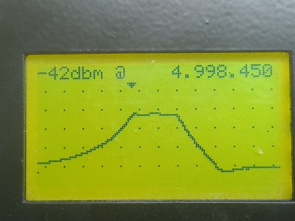
QER filter as swept on the Antuino
The Bandpass filter
We have traditionally used double tuned circuits. It kept away the broadcaster on the image frequencies, well, mostly. There were always the stations and birdies that tuned in the wrong direction. The image suppression was just about 50 dB. Some of the even more respectable amateur radio manufacturers of American heritage have chosen to use just a doubly tuned filter in the front-end. This is a false economy. Addition of another capacitor and inductor makes this a triple tuned circuit with far better results. You can go crazy and make a four section or even a higher section bandpass filter but the performance gains will diminish for two reasons:-
-
- For more than 80 dB of out-of-band rejection you will need to control leakages around the filter rather than through it. You will have to box up the filter, use good cabling, shield each inductor from the other with an interstage shield, etc.
- With each stage, the losses mount. The narrower the filter, the lossier it is. It has to do with the ratio of the loaded to unloaded Q of the filters. With that in mind, here is yet another distraction on designing the band-pass filters. I have simplified it to the extreme. But here it is all the same.
-
 Let’s start.
We have all heard of the Q factor (the Quality) for toroids, inductors, etc. Q is just the ratio of Center frequency to the bandwidth of a band pass filter. For instance, if you wanted a 100 KHz bandwidth from a 7 Mhz filter, that would be a Q of 7000/100 = 70. This is the loaded Q of the filter. As we discussed earlier, filters are specified at certain terminations. In our case, we are looking at a bandwidth of 500 KHz,
So, the QL = 14 (7000/500). (Eq 1)
What makes the Q high or low? It is the losses in a tuned circuit. Losses can be approximated by a parallel resistance too. This is where the impedance comes into play. Higher the impedance of the resonator in a filter, narrower the bandwidth. There is a simple formula to calculate that :
Rp = X * Q [ here X is the reactance of the inductor]
Let’s assume that we will use a 2 uH inductor, its’ reactance will be
X = 6.28 * Frequency * Inductance = 87.92 ohms [or more accurately +j87.92]
(We calculate reactance as an imaginary number, not important in this case)
Rp = X * Q = 87.92 x 14 = 1232 ohms.
This must be the impedance of each of our resonators. To resonate this at 7.1 MHz, we will need 250 pF capacitors in parallel to the inductor.
Next, we choose coupling capacitors. They are given as:
C = K x (Co / QL)
Here Co is the 250 pF capacitor used to resonate the inductor, K is a magic number. Different types of bandpass filters will provide different numbers, they relate to the polynomials the filters describe. Just trust me and use 0.7 here.
C = 0.7 x (250pf /14) = 12.5 pF
Instead, we will just use 10 pF.
There is a subtle detail now, the coupling capacitors add to the total capacitance seen by the inductors decreasing their effective frequency of resonance, we will need to reduce the 250 pf parallel capacitance by 25 pF to bring the resonance back to 7.1 MHz. So, each parallel capacitance is now 220 pF, this is excellent as we can buy 220 pF capacitors.
Let’s start.
We have all heard of the Q factor (the Quality) for toroids, inductors, etc. Q is just the ratio of Center frequency to the bandwidth of a band pass filter. For instance, if you wanted a 100 KHz bandwidth from a 7 Mhz filter, that would be a Q of 7000/100 = 70. This is the loaded Q of the filter. As we discussed earlier, filters are specified at certain terminations. In our case, we are looking at a bandwidth of 500 KHz,
So, the QL = 14 (7000/500). (Eq 1)
What makes the Q high or low? It is the losses in a tuned circuit. Losses can be approximated by a parallel resistance too. This is where the impedance comes into play. Higher the impedance of the resonator in a filter, narrower the bandwidth. There is a simple formula to calculate that :
Rp = X * Q [ here X is the reactance of the inductor]
Let’s assume that we will use a 2 uH inductor, its’ reactance will be
X = 6.28 * Frequency * Inductance = 87.92 ohms [or more accurately +j87.92]
(We calculate reactance as an imaginary number, not important in this case)
Rp = X * Q = 87.92 x 14 = 1232 ohms.
This must be the impedance of each of our resonators. To resonate this at 7.1 MHz, we will need 250 pF capacitors in parallel to the inductor.
Next, we choose coupling capacitors. They are given as:
C = K x (Co / QL)
Here Co is the 250 pF capacitor used to resonate the inductor, K is a magic number. Different types of bandpass filters will provide different numbers, they relate to the polynomials the filters describe. Just trust me and use 0.7 here.
C = 0.7 x (250pf /14) = 12.5 pF
Instead, we will just use 10 pF.
There is a subtle detail now, the coupling capacitors add to the total capacitance seen by the inductors decreasing their effective frequency of resonance, we will need to reduce the 250 pf parallel capacitance by 25 pF to bring the resonance back to 7.1 MHz. So, each parallel capacitance is now 220 pF, this is excellent as we can buy 220 pF capacitors.
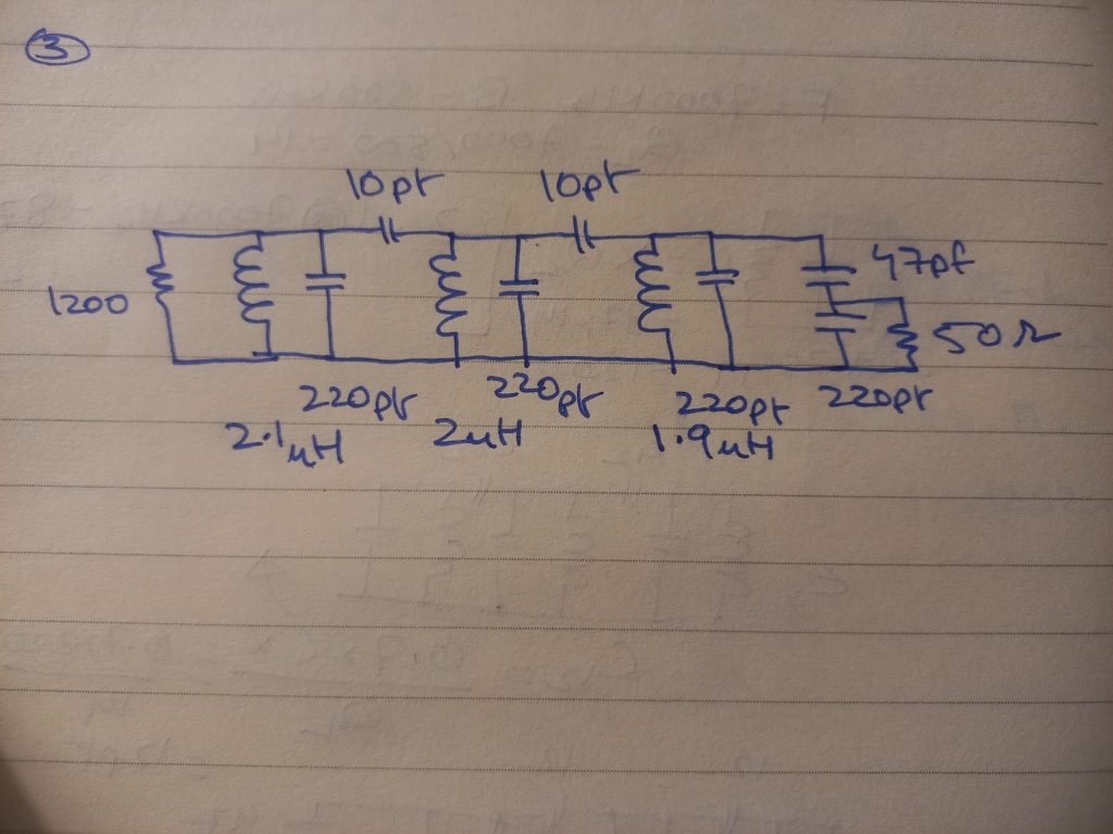
Bandpass filter, Designed.
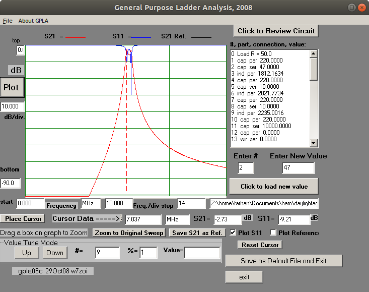
Bandpass filter simulated on GPLA
3D printed toroids
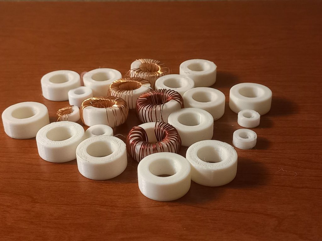 Yet another digression, this one will save you money … You can 3D print toroids!! We experimented with various sizes and finally landed up with 1 inch outer dimension toroids that reports a Q of about 150. Pretty reasonable for toroids that are almost free. You can print 10 of them at a time on the a home 3D printer. This was a big learning from this project.
We have used them in the bandpass filter as well as the low pass filter. They perform pretty well. To calculate the inductance, you have to square the number of turns and multiply with two.
Inductance [in nano henry] = 2 * (number of turns)2
Yet another digression, this one will save you money … You can 3D print toroids!! We experimented with various sizes and finally landed up with 1 inch outer dimension toroids that reports a Q of about 150. Pretty reasonable for toroids that are almost free. You can print 10 of them at a time on the a home 3D printer. This was a big learning from this project.
We have used them in the bandpass filter as well as the low pass filter. They perform pretty well. To calculate the inductance, you have to square the number of turns and multiply with two.
Inductance [in nano henry] = 2 * (number of turns)2
The Receiver, then
Here is the receiver part of the radio in all its glory.
Receiver Portion. Click on it for a larger version
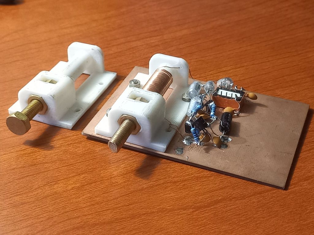 The VFO is another 3D printed part. Instead of hard to find variable capacitors, we use a variable inductor to tune the band. After all this is 2022. Slow motion drives are hard to find. They are messy to install, they exhibit backlash. Instead, we used a simple 3D printed PTO. It is essentially an air inductor about 5 cm long that can be horizontally mounted on the PCB with four M3 screws. It has two slots where you can insert nuts for 1/4-20 screws. A nice long brass 1/4-20 bolt is the main tuning element that moves in and out, guided by the two nuts held firmly in their slots. It provides around a decent, 25 KHz tuning per turn. It took 40 turns of 22 swg enamelled wire to fill the former end to end. The tap is at 10 turns. The 3D printed PTO is really easy to build. It prints in 15 minutes. It is dead stable at 2 MHz. To net to the exact frequency range, you can add or remove turns on the PTO former.
Three polystyrene capacitors of 470 pF each, in parallel, brought the tuning in the range of 2 MHz. A serendipitous advantage of 2 MHz PTO that tunes upwards is that a regular frequency counter can be used for accurate tuning.
A 78L09 was used as the PTO’s voltage regulator. A simpler choice would have been to use a 9.1v Zener diode. We didn’t. The zener regulator works by sinking current that the VFO isn’ consuming. This current converts to heat which can drift the VFO. On the other hand, if we reduced the current, the Zener would starve and turns noisy and the regulation would suffer too. Instead, the free running VFOs are best powered by 78L09. They hardly sink any current, they are noise free if they are properly bypassed both at the input and the output. For a VFO you must also bypass it at audio to remove any hum modulation. A 1uf electrolytic capacitor mounted very close to the terminal output pin is recommended.
The PTO has the minor visual disturbance of a knob that comes out and goes back in. It is best to leave it tightened against the chassis when not in use or that take it away with you to prevent other prying hams from using the radio!
We use a low power single JFET as a buffer. The cascode mixer and the transmit mixer hardly need any driving power and hence the bias current is kept low.
The PTO is built with just the component leads themselves. A box made from thin copper sheeting is soldered around it to keep it thermally stable and prevent the RF from the transmitter, etc from coupling into the PTO. Without the shielding, there was a transmit spur at 8 MHz, probably from the PTO’s 4th harmonic. It went away with the shielding and it was never fully investigated.
The VFO is another 3D printed part. Instead of hard to find variable capacitors, we use a variable inductor to tune the band. After all this is 2022. Slow motion drives are hard to find. They are messy to install, they exhibit backlash. Instead, we used a simple 3D printed PTO. It is essentially an air inductor about 5 cm long that can be horizontally mounted on the PCB with four M3 screws. It has two slots where you can insert nuts for 1/4-20 screws. A nice long brass 1/4-20 bolt is the main tuning element that moves in and out, guided by the two nuts held firmly in their slots. It provides around a decent, 25 KHz tuning per turn. It took 40 turns of 22 swg enamelled wire to fill the former end to end. The tap is at 10 turns. The 3D printed PTO is really easy to build. It prints in 15 minutes. It is dead stable at 2 MHz. To net to the exact frequency range, you can add or remove turns on the PTO former.
Three polystyrene capacitors of 470 pF each, in parallel, brought the tuning in the range of 2 MHz. A serendipitous advantage of 2 MHz PTO that tunes upwards is that a regular frequency counter can be used for accurate tuning.
A 78L09 was used as the PTO’s voltage regulator. A simpler choice would have been to use a 9.1v Zener diode. We didn’t. The zener regulator works by sinking current that the VFO isn’ consuming. This current converts to heat which can drift the VFO. On the other hand, if we reduced the current, the Zener would starve and turns noisy and the regulation would suffer too. Instead, the free running VFOs are best powered by 78L09. They hardly sink any current, they are noise free if they are properly bypassed both at the input and the output. For a VFO you must also bypass it at audio to remove any hum modulation. A 1uf electrolytic capacitor mounted very close to the terminal output pin is recommended.
The PTO has the minor visual disturbance of a knob that comes out and goes back in. It is best to leave it tightened against the chassis when not in use or that take it away with you to prevent other prying hams from using the radio!
We use a low power single JFET as a buffer. The cascode mixer and the transmit mixer hardly need any driving power and hence the bias current is kept low.
The PTO is built with just the component leads themselves. A box made from thin copper sheeting is soldered around it to keep it thermally stable and prevent the RF from the transmitter, etc from coupling into the PTO. Without the shielding, there was a transmit spur at 8 MHz, probably from the PTO’s 4th harmonic. It went away with the shielding and it was never fully investigated.
The Transmitter

Click on the image for a larger picture

Full circuit (click to enlarge)
Leave a Reply